Train a person detection model to run on a microcontroller (part two)

Training & converting the model

MACHINE LEARNINGIOT

3/19/20237 min read

Introduction

In the first part of this series, we discussed the process of collecting and preparing the data needed to train a person detection model. Now that we have our dataset ready, it's time to dive into the process of training the model using TensorFlow and subsequently converting it to TensorFlow Lite (TFLite) for deployment on mobile and edge devices. In this second part, we will assume that the data is already available, and we will follow a reference notebook hosted on GitHub to walk you through each step.

Model Architecture selection

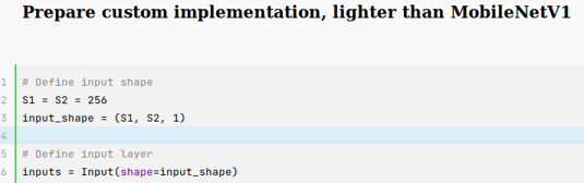
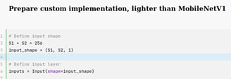
Considering the constraints of the deployment environment, resource-intensive models such as VGG16/19, Xception, and their counterparts are not suitable choices. A more fitting alternative is MobileNetV1, which offers a lightweight and efficient architecture specifically designed for mobile and edge devices. MobileNetV1 is a highly efficient convolutional neural network architecture designed specifically for mobile and embedded vision applications. It was introduced by Google researchers in 2017 as a lightweight alternative to more computationally intensive models like VGG and ResNet. The main innovation behind MobileNetV1 is the use of depthwise separable convolutions, which significantly reduce the number of parameters and computational complexity compared to traditional convolutional layers. Depthwise separable convolutions consist of two steps: depthwise convolutions and pointwise convolutions. In depthwise convolutions, each input channel is convolved with its own set of filters, while pointwise convolutions combine the outputs of depthwise convolutions using 1x1 convolutions. This results in a model that is smaller in size, faster to run and has lower memory requirements. You can easily download a MobileNet model (with weights), like this:

Take note that we are adapting the top layer of the model to accommodate our specific use case, which involves only two classes: person and no-person. By making this modification, the model contains 3,229,889 parameters, amounting to more than 3 million. Such a model can be too heavy for a microcontroller. We can try to rewrite the model from scratch, to reduce this number, this is an iterative approach, as you need to check the model accuracy to see if it fits your need. I decided to write my custom model, with a structure similar to the original MobileNet, achieving a model with around 250000 parameters. It is also essential to consider the input shape, specifically the image size when designing a model for resource-constrained environments. Ideally, you should aim to work with smaller image sizes, such as 256x256 pixels or less. Smaller image dimensions can help reduce the computational complexity and memory requirements of the model. Additionally, you may want to consider using grayscale images instead of RGB images. Grayscale images contain only one channel, as opposed to the three channels (red, green, and blue) in RGB images. By using grayscale images, you further reduce the amount of data the model needs to process, leading to a more lightweight and efficient model. For instance, a 256x256 grayscale image requires 65,536 bytes of memory (256x256x1), while the same image in RGB format would require 196,608 bytes (256x256x3). This reduction in memory requirements can greatly impact the performance and efficiency of your person detection model, especially when deploying on mobile or edge devices with limited resources. I have done an attempt with 128x128x1 first, and 256x256x1 and I successfully deployed both models into my ESP32. You can easily modify the input shape by modifying the following cell:

S1 and S2 are the variables to change.

The training process

To train the person detection model effectively, I have incorporated several data augmentation techniques that help improve the model's ability to generalize and recognize people under varying conditions. These augmentation functions include adjustments to saturation, the addition of noise, gamma correction, and more. The custom training loop is designed to handle the balance between the two classes: person and no-person. For a given batch, it selects half of the batch size's images containing a person and the other half without a person. This approach ensures a balanced distribution of samples during the training process, which can help the model learn to distinguish the two classes more effectively. After selecting the images, the training loop applies random augmentation functions to the images, generating the input (X) and the corresponding labels (Y). This augmented data is then fed into the model using the train_on_batch function. The primary focus of my custom training loop is flexibility, rather than efficiency. By implementing the training process this way, I can easily adjust the balance between classes and the augmentation functions applied, allowing for fine-tuning and experimentation to achieve the best possible results for the person detection model. I have been able to achieve an accuracy close to 90% on the validation test.

A note on the environment setting and repo link

To simplify the process of setting up the environment, a requirements.txt file is provided in the repository. You can use this file to install the necessary dependencies for the project. Additionally, I have included a Dockerfile in the repository, which allows you to build a Docker container based on the tensorflow/tensorflow:latest-gpu image. This container is pre-configured to start a Jupyter Notebook on port 8889 when launched. To build and start the Docker container, you can refer to the build_docker.bash and start_docker_gpu.bash scripts. Please note that to fully benefit from the GPU-enabled TensorFlow image, you need to have a compatible GPU installed on your system. The main advantage of using Docker in this scenario is that it helps avoid potential issues with the CUDA drivers on your host machine.
The repo for this training part is available here.

Converting the model into TF-Lite (Quantization)

TensorFlow Lite (TFLite) is a lightweight and efficient framework designed for deploying TensorFlow models on mobile and embedded devices with limited resources. A standard TFLite model typically delivers the same results as a full TensorFlow model, making it an ideal choice for edge deployments without sacrificing accuracy. However, to further optimize the model for size and computational efficiency, quantization can be applied during the conversion process. Quantization is a technique that reduces the precision of the model's weights and biases, resulting in smaller model size and faster inference times. This step is especially important when deploying the model on microcontrollers, where resources are highly constrained. It's important to note that quantization can potentially affect the accuracy of the model. However, by using techniques like post-training quantization, the impact on accuracy can be minimized. In this case, the model is quantized after training, preserving the original model's accuracy as much as possible. Here's the code snippet to create a quantized TFLite model:

The crucial aspect of this code is that the representative dataset is passed to the converter. This allows the quantization process to be performed correctly, minimizing the impact on the model's accuracy. In this example, both the input and output remain as float values since the ESP32 microcontroller supports float operations. However, if you're targeting a microcontroller that doesn't support floating-point operations, you may need to convert the input and output to integers as well.
Let's focus a bit more on what quantization is. Quantization is a technique used to reduce the numerical precision of a model's weights, biases, and activations, thereby reducing its memory footprint and computational requirements. Quantization typically involves converting floating-point values to lower-precision representations, such as integers. This is achieved by using a linear transformation that consists of a scale and an offset (also called zero-point). The scale represents the range of values, while the offset defines the shift applied to the data. The combination of scale and offset allows for preserving the original data distribution as closely as possible while using a lower-precision format. Here's a simple example of the quantization process:

First, the minimum and maximum values of the data to be quantized are determined.
Then, the scale and offset are calculated based on the data range and the target integer precision (e.g., 8-bit integers).
Finally, the floating-point values are transformed using the scale and offset, resulting in the quantized integer representation.

In the code snippet provided earlier, the line converter.representative_dataset = load_grayscale_images plays a crucial role. Without this line, the quantization process defaults to 'dynamic range quantization,' which means only the weights of the model are converted from floating-point to integer representations. This type of quantization is sufficient for reducing the model size by a factor of 4, as integer values typically require less storage space compared to floating-point values. However, by providing a representative dataset using the converter.representative_dataset attribute, the quantization process can be more comprehensive, encompassing not only the weights but also the activations. This approach results in a more optimized model, with improved inference speed and potentially better accuracy preservation compared to dynamic range quantization alone. If you want to can go even further, adding the following:

A simple quantization example

Let's try to make it even clearer, with a simple example, let's suppose we have a network with two fully connected layers, an input which is a scalar (1x1, for simplicity). We will have an input processing, to convert from float to integer, let's assume our input value is x = 2.0, and the input scale and offset are x_scale = 0.05 and x_offset = 100. We preprocess the input by converting it to an 8-bit integer using the scale and offset: x_quant = round((x / x_scale) + x_offset) = round((2.0 / 0.05) + 100) = 140 In the first forward pass, we perform the pure integer computation: y_quant = x_quant w_quant + b_quant. Where w_qaunt and b_quant are the quantized weights. Then we pass the output to a RELU, achieving: y1_quant_relu = max(y1_quant, zero_point) . The second forward pass is similar, but with different weights: y2_quant = y1_quant_relu * w2_quant + b2_quant. Then for the output layer, we can potentially go back to float, like this: y2 = y2_scale * (y2_quant - y2_offset).

Wrap up

Quantization is not a straightforward topic, but at the core, it is a way to pass from a larger domain (float) to a smaller one (unsigned integer), it is a simple linear transformation as we have seen above. Here is the official documentation about it, while here, is my notebook.

The above image, shows the results, for some sample images, of the original model, quantized model, and TFLITE model without quantization. It is interesting to see how the quantized model is not far from the non-quantized ones. The notebook then ends with the following cell:

'xxd' transform the quantized TFlite model into a char array. This is the foundation of the next article, where the model will be deployed into the ESP32.

Like that, we are forcing the conversion to be uint8 only, including input & output. If you have an ESP32, you don't need it, but you can definitely add it.

How scale and offset are computed?

To clarify the process of converting floating-point values (4 bytes) to uint8 (1 byte) using the linear transformation formula y_uint = x_float * scale + offset, consider the following example: We want to transform our input, with float values ranging from -1 to 1 (inclusive), into uint8 values. This linear transformation requires calculating the scale and offset values through the system below, it is interesting to notice that, if the float values are not negative the offset is 0.